Monte Carlo Simulation
Andrew Agathangelou, Technical Director, Driver Trett UK assesses the usefulness of statistical techniques to assess the probability and risk associated with achieving a defined completion date.
In 2005, I was providing consultancy services to a developer regarding the construction of a major UK retail development. The project was beset with many delays and was running a year late at that point.
Each month, the developer received a progress report which included a forecast of the earliest date the project was likely to finish, based upon:
A) Progress achieved to date; and
B) Completion of the remaining works in line with the originally programmed periods and sequence of works.
Whilst a conventional progress forecast of this manner is a useful method of indicating the status of the works at a given point in time, it is not necessarily an indicator of the date a project might finish.
This is because this type of forecast method does not use the historical progress data achieved to date to calculate a progress trend, and then project the trend going forward to establish the likely completion date. Neither did the exercise, in this instance, consider the probability of the remaining construction activities being achieved in line with their original planned durations which were, at best, only estimates of the expected durations based on previous experience.
Given this uncertainty, and the fact that the project continued to fall even further behind every month, the developer posed the following question: what date could the shopping centre be opened with 99% certainty?
Having been tasked with providing the answer, I researched my options and was directed to conducting a Monte Carlo simulation using an additional software package they supplied. The Monte Carlo method is a probability simulation which is used to understand the impact of risk and uncertainty regarding project management, cost, or progress forecasting models.
The simulation I employed required an estimation of the minimum duration, most likely duration and the maximum duration for some or all of the construction activities in the programme for the remaining works. For the purposes of the exercise I undertook, I chose only those activities that lay directly on the longest (critical) path of the works, which determined the project’s overall duration and completion date.
To illustrate how, in principle, the Monte Carlo simulation works, I will use a hypothetical project in which the concrete frame is one of the key critical activities determining overall completion.
Figure 1
|
Construction Activity
|
Minimum Time
|
Most Likely Time
|
Maximum Time
|
|
Concrete Frame Area 1
|
47 weeks
|
55 weeks
|
65 weeks
|
In this example, I have estimated the following minimum, maximum and most likely durations for the concrete frame based upon personal experience: (Figure 1).
Figure 2
|
Construction activity
|
Possible Duration (Time)
|
|
Concrete Frame Area 1
|
47 - 50 weeks - minimum
|
|
|
50 - 55 weeks – most likely
|
|
|
55 - 58 weeks
|
|
|
58 - 62 weeks
|
|
|
62 - 65 weeks - maximum
|
Having assigned the minimum, maximum and most likely durations for the concrete frame, a range of other possible durations are generated by the simulation which sit within the specified minimum and maximum periods, as shown in figure 2.
The establishment of the range of possible durations makes it possible for the Monte Carlo simulation to use statistical techniques to establish the likelihood or probability of the duration value occurring.
Figure 3
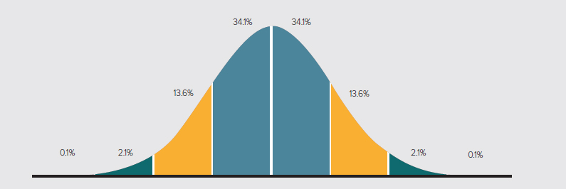
In many situations where data is collected on a large scale, for example exam results, the distribution of the results will often follow what is called a normal distribution curve where the apex of the curve represents the mean (average). The distribution of the results will spread out either side of the mean value, as illustrated below. This spreading out or deviation from the mean is called the ‘standard deviation’ and measures the spread of the results. A small standard deviation indicates that the data or values obtained are tightly clustered around the mean - the normal distribution curve will be taller. A larger standard deviation indicates that the data or values are more spread out either side of the mean – the normal distribution curve will be wider and flatter (Figure 3).
A characteristic of a normal distribution curve is that 68% of the values (whether they be exam grades or estimated construction durations) can be found within one standard deviation from the mean, as illustrated by the teal area in the diagram above. Further, 95% of the values can be found within 2 standard deviations from the mean – the first standard deviation is the blue area illustrated above, and the second standard deviation is illustrated by the yellow area. These two standard deviations combined account for 95% of the data or values under consideration.
Back to our example, for each of the above duration ranges, the Monte Carlo simulation would generate a minimum of 500 random numbers whose value fell within the range specified. For example, for the 47 to 50 weeks duration range the Monte Carlo simulation would generate 500 random numbers whose value would be either 47, 48, 49 or 50. Likewise, the 50 to 55 week duration range the simulation would similarly generate 500 random numbers whose value would be either 50, 51, 52, 53, 54 or 55. This generates a normal distribution curve for each of the concrete frame duration ranges, with each normal distribution curve containing the values of 500 random numbers whose values fall between the specified duration ranges.
Figure 4

Taking the duration range of between 47-50 weeks again as an example, a minimum of 500 random numbers were generated whose values were either 47, 48, 49 or 50. The Monte Carlo simulation records the frequency with which each number occurred in the simulation. In other words, the simulation records the number of times the number 47 occurred out of a total of 500, the number of times the number 48 occurred out of a total of 500 and so on. With 500 random numbers generated with values between 47 to 50 the simulation can calculate the mean value, and the two standard deviations from the mean in which 95% of the values are found as illustrated on page 26 (Figure 4).
Likewise for the duration range of between 50 and 55 weeks, the simulation would generate 500 random numbers whose values were either 50, 51, 52, 53 or 55, and the frequency with which each these numbers occurred. This continues for the duration range of 55-58 weeks and so on.
Figure 5
|
Time (value)
|
Number of Times (out of 500)
|
Percent of Total
|
|
47 weeks - minimum
|
10
|
2%
|
|
50 weeks
|
150
|
30%
|
|
55 weeks – most likely
|
225
|
45%
|
|
58 weeks
|
375
|
75%
|
|
62 weeks
|
470
|
94%
|
|
65 weeks - maximum
|
495
|
99%
|
The table above illustrates the number of times each of the specified durations occurred in the simulation, and thereby the likely probability of it being achieved;
If we take the minimum period of 47 weeks for example, the value 47 appeared 10 times out of the 500 random numbers generated, or 2% of the total. Therefore, the probability of the 47-week duration being achieved or occurring is 2%.
It can be seen in the above example that what was considered one of the most likely durations before the simulation was undertaken, 55 weeks, only had a 45% probability of being achieved i.e. less than a 50/50 chance. If we assume that the duration with a 75% probability of being achieved will be the most likely duration, the most likely duration will be 58 weeks.
Running similar simulations involving all the selected critical path activities for my retail project, generated a range of possible outcomes for the overall project duration, as follows:
Figure 6
|
Overall Project Duration
|
Probability
|
|
105 weeks
|
2%
|
|
112 weeks
|
30%
|
|
125 weeks
|
45%
|
|
132 weeks
|
75%
|
|
147 weeks
|
85%
|
|
150 weeks
|
99%
|
It can be seen from figure 6 that the overall project duration which could be achieved with 99% probability or certainty would be 150 weeks, with 132 weeks being the most likely overall duration (based on the 75% result set out in the table above).
Going back to the real question posed by the developer of the West London shopping centre in 2005, I ran the Monte Carlo simulation several times and obtained very similar results on each occasion. I reported to the developer that if it wanted to open the shopping centre with 99% certainty, the opening date would be 24 October 2008. The developer was taken aback because the reported forecast delay to the works was significantly less than this, with a far earlier completion date. The shopping centre opened some three years after the simulation was run – on 30 October 2008!